2 Dataset

2.1 Technical description

The dataset we use is called modeled exposure to particulate matter air pollution, that aggregates the concentration of the fine particulate matter (PM 2.5) in 194 over the world. In particular, it includes the annual concentration of PM 2.5 in 194 countries, with breakdown for urban and rural areas. The dataset is authored by the World Health Organization (WHO). In general, to obtain estimates of PM 2.5 levels, the concentration of PM 2.5 is measured from fixed-site monitors located within metropolitan areas. The value of PM 2.5 in a given area can be obtained by averaging the measurements of monitors in this area.

Our dataset includes the average annual PM 2.5 concentration on 194 states from 2010 to 2019. Apart from the average value over the country, the dataset also records the averages on four different area types: urban, rural, cities and towns. The dataset consists of 34 variables in total. Not all of them will be valuable to us, but relevant features include country, location (continent), period (year), area type (detailed below), and value (PM 2.5 concentration). There are 9450 observations, each recording the average annual concentration of PM 2.5 for a specific area type (urban, rural, cities, towns, total) of one of the 194 states in the world.

We obtain the data from the WHO official website. A CSV file can be downloaded from here. The file is ready-to-use, requiring only a “read.csv” function to be loaded into RStudio. We will perform data cleaning (eliminating redundant variables and dealing with NAs) and analysis using this file.

2.2 Research plan

The data provides us with comprehensive information about the mean, minimum, and max PM2.5 at each residence area type, country, continent from 2010 to 2019. Here are some ways that I’m going to use to analyze the data based on our needs.

Pre-processing:
1. Remove unneeded value and handle NaN value.
2. Transform the data for later use by applying pivot_longer(), mutate(), etc.
Analyze air quality change over time:
1. Use time series line chart to plot PM2.5 change from 2010 to 2019, smooth the plot to see the general trend. This can be done in geom-line() function.
2. Create multiple box charts that shows min, max, mean value for each year and each continent in facet graph using facet_wrap().
3. Create a histogram that shows the average PM2.5 for each country and continent.
Analyze air quality change over location:
1. Create a Heatmap using geom_tile to show country differences for PM2.5 and highlight those outliers.
2. Use bar chart to show the average and range of PM2.5 per continent and country.
Analyze air quality change over resident type (urban, rural, cities, towns):
1. Visualize the resident type difference per continent by evaluating the average PM2.5 in the facet graph using ggplot and facet_wrap().
2. Plot the average PM2.5 per continent per resident type as a scatter plot to show if the PM2.5 are significantly different across all resident types.
3. Create a ggalluvial plot over each resident type and year to show the value change for each resident type.
Putting it all together, there are 3 dimensions that we are going to analyze the data, at the end, based on what we observe from the visualizations above, we will use any package that we learned from class to dive deeper into the detail to analyze the abnormality or general trends to validate our hypothesis and make the analysis comprehensive.

2.3 Missing value analysis

Let’s look at our data and understand it. We only have 1 dataset with 34 columns and 9450 rows. We first check if there are any columns that have no useful information for our analysis and select the ones that are useful for us.

The second step is to check if the remaining columns have any missing or incorrect values and adjust them. Here are the breakdown steps:

Code

# import
library(readr)
library(dplyr)


Attaching package: 'dplyr'

The following objects are masked from 'package:stats':

    filter, lag

The following objects are masked from 'package:base':

    intersect, setdiff, setequal, union

Code

library(ggplot2)
library(tidyr)

# read csv
data <- read_csv("data_pollution.csv")

Rows: 9450 Columns: 34

── Column specification ────────────────────────────────────────────────────────
Delimiter: ","
chr  (14): IndicatorCode, Indicator, ValueType, ParentLocationCode, ParentLo...
dbl   (4): Period, FactValueNumeric, FactValueNumericLow, FactValueNumericHigh
lgl  (15): IsLatestYear, Dim2 type, Dim2, Dim2ValueCode, Dim3 type, Dim3, Di...
dttm  (1): DateModified

ℹ Use `spec()` to retrieve the full column specification for this data.
ℹ Specify the column types or set `show_col_types = FALSE` to quiet this message.

Code

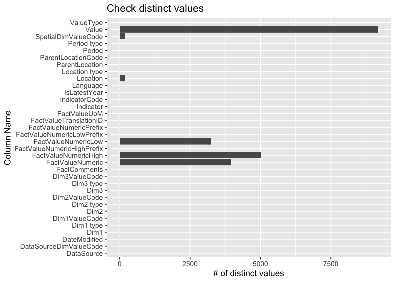
# count distinct values
distinct_counts <- data %>% summarise_all(n_distinct)

long_data <- pivot_longer(distinct_counts, cols = everything(), names_to = "ColumnName", values_to = "DistinctCount")

# plot the number of distinct values per column in our dataset
ggplot(long_data, aes(x = ColumnName, y = DistinctCount)) +
  geom_bar(stat = "identity") +
  coord_flip()+
  labs(x = "Column Name", y = "# of distinct values", title = "Check distinct values")

We can see a lot of columns have a few distinct value, let’s check if they equals 1 or 0, if yes, then we may need to remove these columns since they don’t contribute to our analysis.

Code

# check insignificant data
insignificant_data <- long_data %>% filter(DistinctCount <= 1)
insignificant_data

# A tibble: 22 × 2
   ColumnName    DistinctCount
   <chr>                 <int>
 1 IndicatorCode             1
 2 Indicator                 1
 3 ValueType                 1
 4 Location type             1
 5 Period type               1
 6 Dim1 type                 1
 7 Dim2 type                 1
 8 Dim2                      1
 9 Dim2ValueCode             1
10 Dim3 type                 1
# ℹ 12 more rows

After double-checking our dataset, we found these data could be removed. We then check the NaN values of the rest of the columns.

Code

# check for NaN
selected_columns <- setdiff(colnames(data), insignificant_data$ColumnName)
selected_data <- data %>% select(all_of(selected_columns))

selected_data

# A tibble: 9,450 × 12
   ParentLocationCode ParentLocation SpatialDimValueCode Location         Period
   <chr>              <chr>          <chr>               <chr>             <dbl>
 1 AFR                Africa         KEN                 Kenya              2019
 2 AMR                Americas       TTO                 Trinidad and To…   2019
 3 EUR                Europe         GBR                 United Kingdom …   2019
 4 AMR                Americas       GRD                 Grenada            2019
 5 AMR                Americas       BRA                 Brazil             2019
 6 EUR                Europe         DNK                 Denmark            2019
 7 EUR                Europe         RUS                 Russian Federat…   2019
 8 EUR                Europe         ESP                 Spain              2019
 9 AMR                Americas       GRD                 Grenada            2019
10 AMR                Americas       GRD                 Grenada            2019
# ℹ 9,440 more rows
# ℹ 7 more variables: IsLatestYear <lgl>, Dim1 <chr>, Dim1ValueCode <chr>,
#   FactValueNumeric <dbl>, FactValueNumericLow <dbl>,
#   FactValueNumericHigh <dbl>, Value <chr>

Code

nan_counts <- sapply(selected_data, function(x) sum(is.nan(x)))

nan_counts

  ParentLocationCode       ParentLocation  SpatialDimValueCode 
                   0                    0                    0 
            Location               Period         IsLatestYear 
                   0                    0                    0 
                Dim1        Dim1ValueCode     FactValueNumeric 
                   0                    0                    0 
 FactValueNumericLow FactValueNumericHigh                Value 
                   0                    0                    0

Missing pattern analysis for numeric columns (no missing data).

Code

library(mi)

Loading required package: Matrix


Attaching package: 'Matrix'

The following objects are masked from 'package:tidyr':

    expand, pack, unpack

Loading required package: stats4

mi (Version 1.1, packaged: 2022-06-05 05:31:15 UTC; ben)

mi  Copyright (C) 2008, 2009, 2010, 2011, 2012, 2013, 2014, 2015 Trustees of Columbia University

This program comes with ABSOLUTELY NO WARRANTY.

This is free software, and you are welcome to redistribute it

under the General Public License version 2 or later.

Execute RShowDoc('COPYING') for details.


Attaching package: 'mi'

The following object is masked from 'package:tidyr':

    complete

Code

x <- missing_data.frame(as.data.frame(subset(data, select=c(FactValueNumeric, FactValueNumericHigh, FactValueNumericLow))))
image(x)

We conclude that there is no missing value in the data we selected.

Code

# Write data to csv
write.csv(selected_data, file = "selected_data.csv")